Let's have a look...
In the video, Shawn recognized that the data on his scatterplot was non-linear. It will be difficult for Shawn to use a linear model to analyze the non-linear data.
Data with a linear association has a constant rate of change throughout the graph. A scatterplot that shows a linear association between the variables is modeled with a straight line. But a scatterplot that shows a non-linear association between the variables cannot be modeled with a straight line because the slope along a curved line changes as you move from left to right.
Although you cannot use a linear model to directly represent non-linear data, there are strategies that allow you to use a linear model to analyze non-linear data.
To do so, you must find a linear association inside the non-linear association by 1) focusing in on a specific part of the data that is linear or 2) ignoring any points that are outliers. Read the tabs to learn about each strategy.
Focusing in on a linear portion of a non-linear association allows you to use a linear model to represent part of the data. You can think of the process as "zooming in" on the linear portion.
You can describe the part of the data you are focusing on using a domain. A domain describes the \( x \)-values. The portion of data being focused on is never described using the \( y \)-values.
When focusing on the linear part of a non-linear set of data, it is important to include as much of the data as possible. Generally, it is acceptable to exclude less than half of the data set.
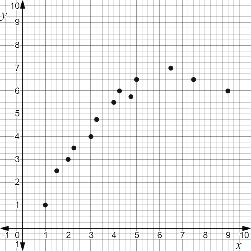
A non-linear scatter plot.
This scatterplot shows a non-linear association.
What portion of the data can be modeled with a straight line? State the domain that has a linear association.
The steps for focusing on a portion of the data that can be modeled with a straight line are shown in the table below. Click each step to learn how to identify and state the domain of the data that has a linear association.
The highlighted section of the data shows a linear association. 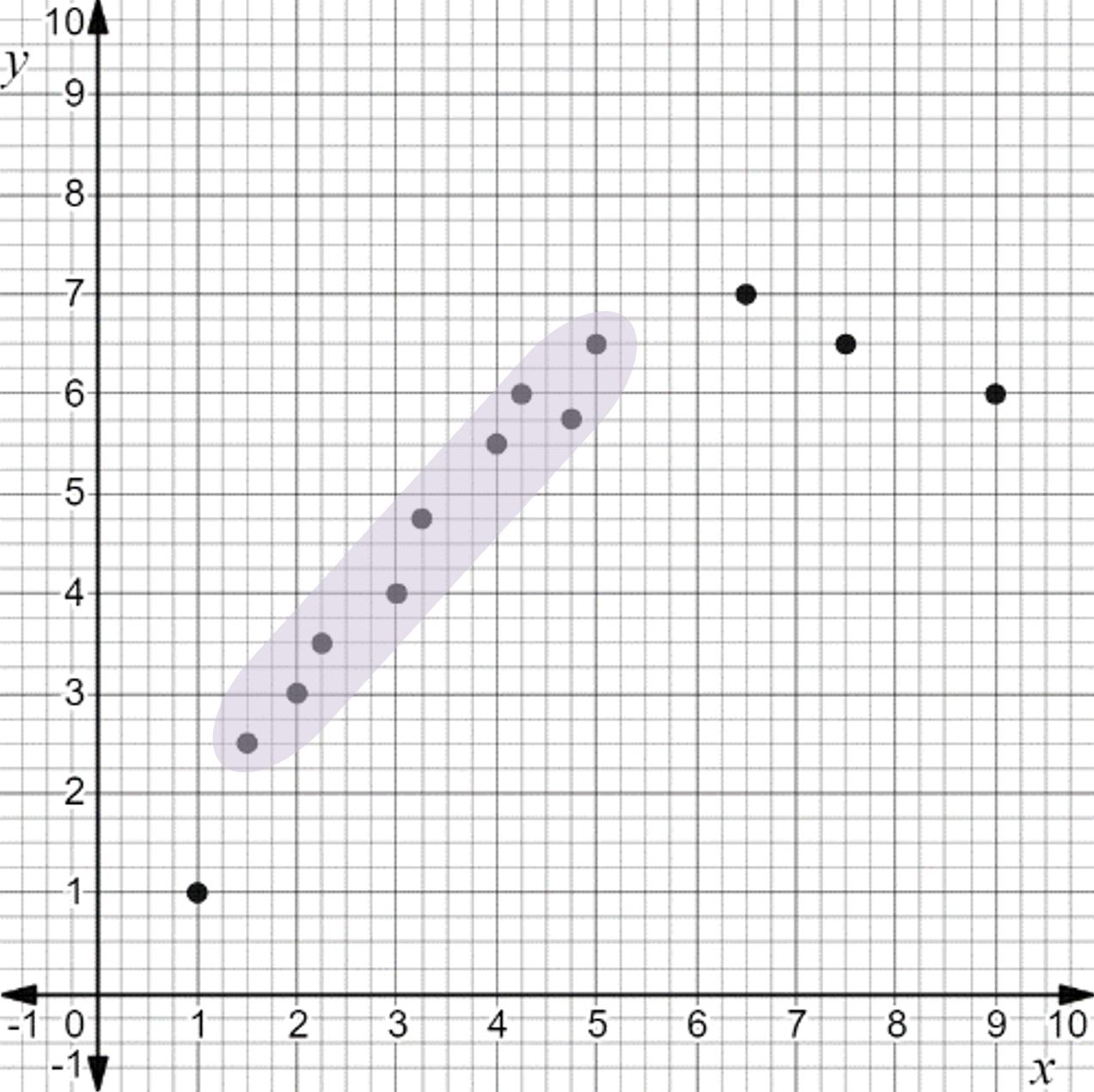
A non-linear scatter plot. The ordered pairs (1.5, 2.5), (2, 3), (2.25, 3.5), (3, 4), (3.25, 4.75), (4, 5.5), (4.25, 6), (4.75, 5.75), and (5, 6.5) are highlighted. |
|
There are 9 data points included in the highlighted section. There are 4 points being excluded. Four is less than half the data, so it is acceptable to use the highlighted section for a linear model. |
|
|
A non-linear scatter plot. The ordered pairs (1.5, 2.5), (2, 3), (2.25, 3.5), (3, 4), (3.25, 4.75), (4, 5.5), (4.25, 6), (4.75, 5.75), and (5, 6.5) are highlighted. The domain of the highlighted section is based on \( x \)-values of the included data points. The highest and lowest \( x \)-values make the domain. These come from the data points that are farthest right and left in the included section. The highest \( x \)-value of the included data is 5. The lowest \( x \)-value of the included data is 1.5. The domain with a linear association is from 1.5 to 5. |
The data in the domain from 1.5 to 5 has a linear association, which means that this portion of the data can be modeled by a straight line.
Outliers are data points that do not fit the general data pattern. Sometimes outliers are not clearly separate from the data pattern, which makes the pattern look non-linear.
Sometimes it is possible to make a non-linear association appear more linear by ignoring one or two outliers. The outliers must be identified by their coordinates.
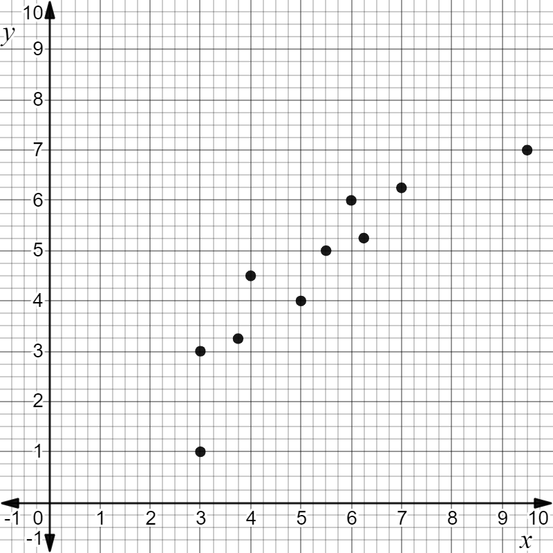
A non-linear scatter plot.
This scatterplot shows a non-linear association.
Which points could be ignored as outliers so that the rest of the data can be modeled with a straight line?
The steps for identifying outliers that can be ignored so that the data can be modeled with a straight line are shown in the table below. Click each step to see it applied to this example.
The highlighted portion of the data shows a linear association. 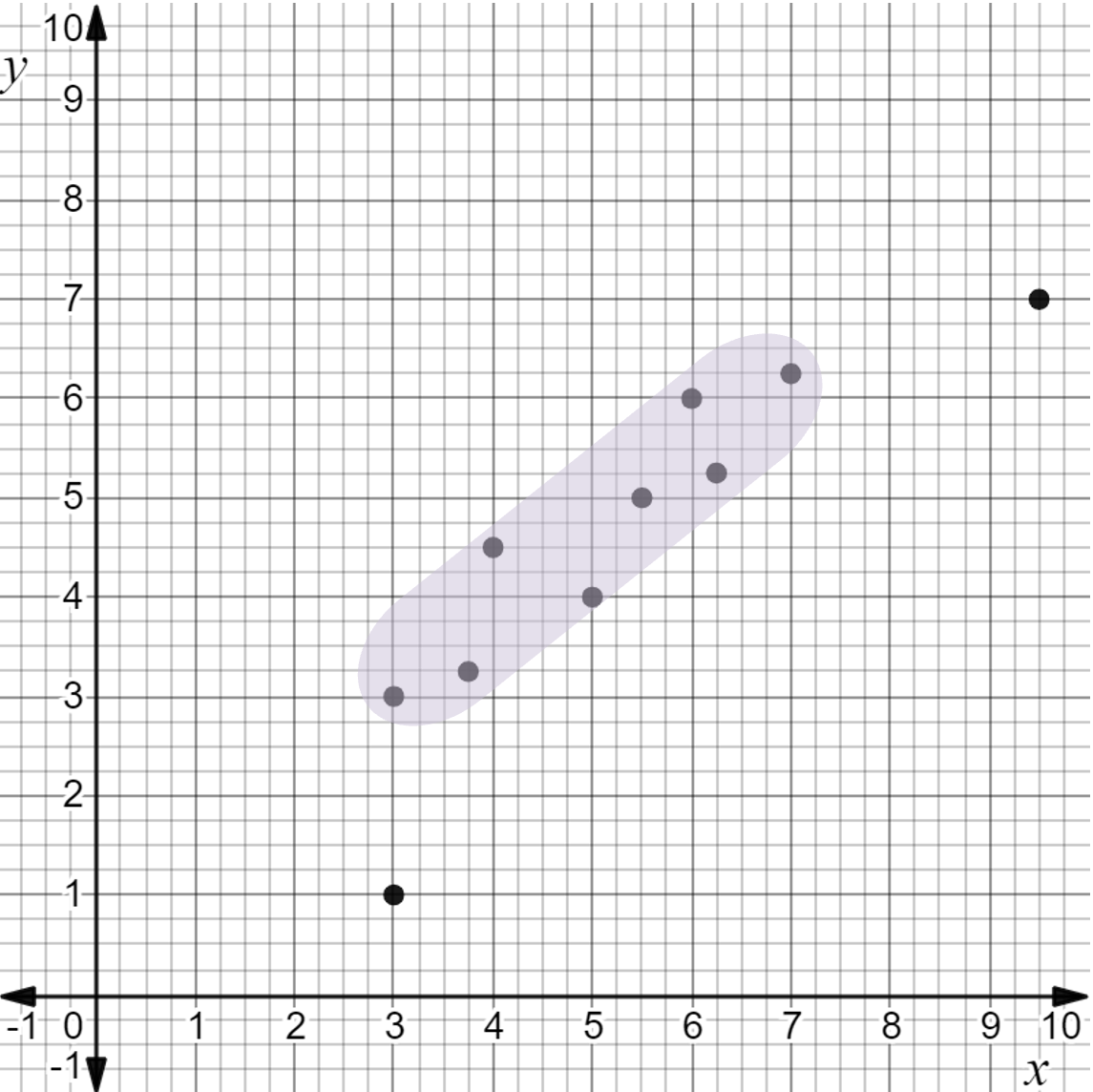
A non-linear scatter plot. The ordered pairs (3, 3), (3.75, 3.25), (4, 4.5), (5, 4), (5.5, 5), (6, 6), (6.25, 5.25), and (7, 6.25) are highlighted. Notice that it is not possible to focus on the domain of the linear section because there is an outlier point with an \( x \)-value in the domain. |
|
There are only two points that are possible outliers. This is an acceptable number of outliers to ignore while creating a linear model. |
|
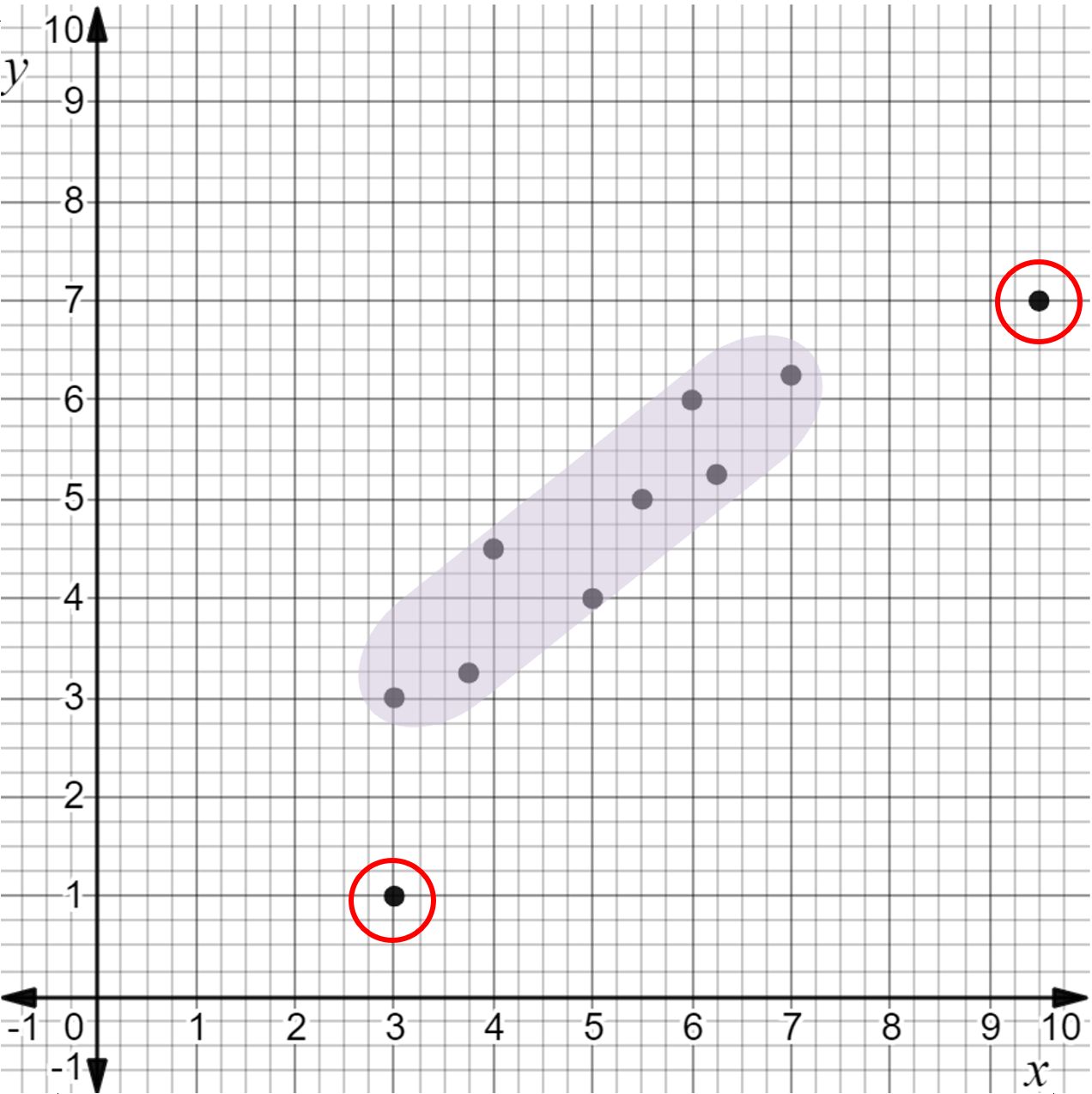
A non-linear scatter plot. The ordered pairs (3, 3), (3.75, 3.25), (4, 4.5), (5, 4), (5.5, 5), (6, 6), (6.25, 5.25), and (7, 6.25) are highlighted and the ordered pairs (3, 1) and 9.5, 7) are circled. The two outlier points are (3, 1) and (9.5, 7). |
The outliers, (3, 1) and (9.5, 7), can be ignored while creating a linear model for the data.
Question
How are the processes of identifying a linear domain or identifying outliers similar? How are they different?
The two processes are similar because both try to keep as much of the data as possible. They are different in that identifying a domain selects a section of the data exactly how it was given. Identifying outliers allows data to be removed.