Let's Review
You used exponential growth functions to model paper folding, population growth, and the growth of investments. The exponential growth function is shown below.

Exponential Growth Function
\( f\left( x \right) = a \cdot b^{x} \)
a = initial value
b = growth factor
x = variable
When modeling exponential growth, \( a \neq 0 \) and \( b > 1 \). In general, the variable x represents a time unit, but it can represent other units as well. The larger the growth factor, the more steeply the graph of the exponential growth function slopes upward. Click on each of these graphs to observe how the growth factor affects the graph.
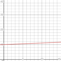
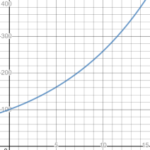

Each of the graphs represents an exponential growth function with an initial value of 100, but with different growth factors. As the growth factor increased, the graph moved up the vertical axis faster.
Question
Look at the graphs presented above. What are the domain and the range for each of these graphs?
All the graphs have a domain of all real numbers. You can substitute any real number into the function and have a real number returned. The range of each of the functions is \( y \geq 0 \).